Know the Differences Between EM-Simulation Numerical Methods
In a closed-loop mathematical system, it often is impossible to represent the complex geometries and boundary conditions of RF/microwave devices and applications. Due to these devices’ diverse material properties and colliding mechanical-electrical properties, however, there is a growing need to grasp, through simulation, their behavior in their actual environments. Computational electromagnetics (CEM) delves into the array of techniques used to efficiently compute approximations to Maxwell’s equations. In doing so, it enables these complex electrodynamic systems to be modeled. While many numerical methods are known to CEM, this article will delve into the numerical methods that are used most commonly in solutions for EM simulation with the latest technologies.
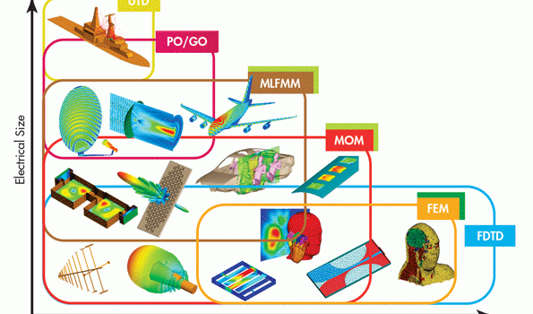
Among the methods used for CEM, for example, are integral-equation solvers, differential-equation (DE) solvers, asymptotic techniques, and other numerical methods (Fig. 1). In the top EM simulation software, which uses integral-equation solving techniques, the methods of moments (MOM) and multilevel fast multipole method (MLFMM) are commonly used. Typically, the numerical methods that use DE solving techniques include the finite-difference time-domain (FDTD), finite-element-method (FEM), and transmission-line-matrix (TLM) methods. In contrast, asymptotic techniques include physical optics (PO), geometric optics (GO), and the uniform theory of diffraction (UTD). The eigen-mode expansion (EME) method is often used for closed resonant systems.
Full article by By Jean-Jacques DeLisle, Microwaves and RF
About the Author
Roger Chu is the Marketing Coordinator at GSAmart, the leading GSA sales and marketing partner for technology companies.